Download the notebook here!
Complete Working Example
In this example we use the CausalForest class from cforest to fit a model on data. With the fitted model we predict effects on new data and visualize these predictions. On top we showcase how one can save and load a fitted model.
[1]:
import numpy as np
from pandas.testing import assert_frame_equal
from cforest.forest import CausalForest
[2]:
from example import simulate
from example import plot_treatment_effect
from example import plot_predicted_treatment_effect

%matplotlib inline
Data
Here we use simulated data. For the sake of simplicity we chose a very simple data generating process using the Neyman-Rubin potential outcome framework.
Treatment effect:
In the Neyman-Rubin potential outcome framework we postulate the existence of so-called potential outcomes. That is, for the outcome we want to measure we assume that, in theory, an individual \(i\) has a (potential) outcome if it were not treated, which we call \(y_i^0\), and a (potential) outcome if it were treated, which we call \(y_i^1\). These potential outcomes exist no matter if the individual was actually treated or not. In reality we only observe one outcome, namely \(y_i\); however, if the individual was treated we get \(y_i = y_i^1\) and otherwise \(y_i = y_i^0\).
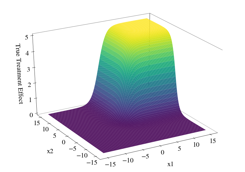
The (individual) treatment effect is defined by \(\tau_i = y_i^1 - y_i^0\), which again cannot be computed since at least one potential outcome is unobservable. In the following we assume that the treatment effect is a smooth function which depends on two covariates and our goal will be to estimate this function. Analytically we can write the treatment effect function as
which (using \(\gamma = 5\) and \(\alpha = 0.9\)) looks as
[13]:
plot_treatment_effect(alpha=0.9, scale=5, figsize=(14, 10))
Simulation strategy:
For (independent) individuals \(i=1,\dots,n\) do:
Simulate (independent) covariates: \(x_{i1}, x_{i2} \sim \mathrm{Unif}(-15, 15)\)
Simulate error terms: \(\epsilon_i \sim \mathcal{N}(0, \sigma^2)\)
Compute untreated potential outcome: \(y_i^0 = 0.5 + 0.1 x_{i1} - 0.1 x_{i2} + \epsilon_i\)
Compute treated potential outcome: \(y_i^1 = y_i^0 + \tau(x_{i1}, x_{i2})\)
Simulate treatment status: \(T_i \sim \mathrm{Bern}(0.5)\)
Compute (observed) outcomes: \(y_i = T_i y_i^1 + (1 - T_i) y_i^0\)
Return: Outcomes \(y_i\), covariates \(x_i = (x_{i1}, x_{i2})\) and treatment status \(T_i\).
Create the data:
[4]:
params = {
    'nobs': 5000,
    'nfeatures': 2,
    'coefficients': [0.5, 0.1, -0.1],
    'error_var': 0.1,
    'seed': 1,
    'alpha': 0.9,
}

X, t, y = simulate(**params)
Estimation (fitting)
Initiate a Causal Forest estimator:
[5]:
cfparams = {
    'num_trees': 40,
    'split_ratio': 1,
    'num_workers': 4,
    'use_transformed_outcomes': False,
    'min_leaf': 5,
    'max_depth': 20,
    'seed_counter': 1,
}

cf = CausalForest(**cfparams)
Fit the model onto the training data:
[6]:
cf = cf.fit(X, t, y)
Prediction
Predict treatment effects for newly observed covariates:
[7]:
newx = np.array([
    [5, -10],
    [-10, 5],
    [-10, -10],
    [5, 5],
    [10, 10]
])

predictions = cf.predict(newx, num_workers=2)
predictions
[7]:
array([0.04468647, 0.1118838 , 0.12054378, 4.83699512, 5.01450885])
[8]:
newx = np.array([
    [5, -10],
    [-10, 5],
    [-10, -10],
    [5, 5],
    [10, 10]
])

predictions = cf.predict(newx, num_workers=2)
predictions
[8]:
array([0.04468647, 0.1118838 , 0.12054378, 4.83699512, 5.01450885])
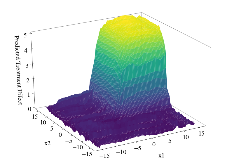
Visualize the predicted surface:
[9]:
plot_predicted_treatment_effect(cf, figsize=(14, 10), npoints=75, num_workers=4)
Saving the Model
To save a (fitted) estimator model we simply call the save method with the filename.
[10]:
cf.save(filename="fitted-example-model.csv", overwrite=True)
Loading a Fitted Model
To load a model we have to iniate a new CausalForest object or use an old one and overwrite the fitted_model their. Here we iniate a new one, load the model which we just saved and assert that the stored models in the two estimators are equal.
[11]:
cff = CausalForest(**cfparams)
cff = cff.load("fitted-example-model.csv")

assert_frame_equal(cff.fitted_model, cf.fitted_model)
Bonus
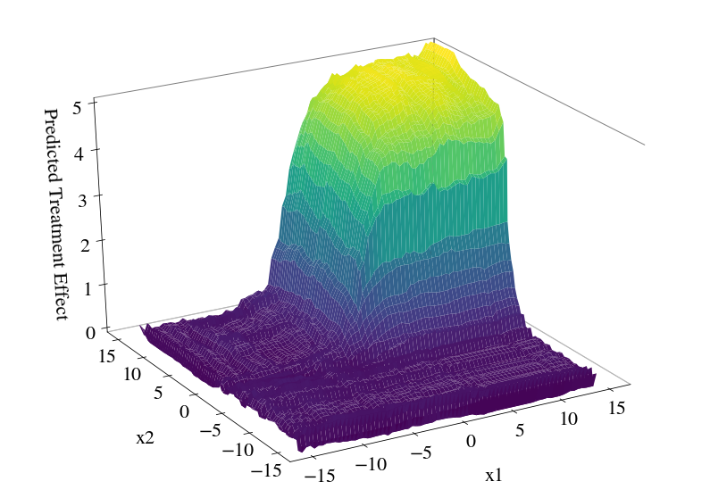
How would the fit look like if we change the splitting criterion? Currently implemented are two splitting criteria.
One, we split at a point on a certain axis if this split will lead to the highest sum over the resulting regions of squared treatment effects weighted by the number of observations. That is, we maximize
This criterion we get by setting use_transformed_outcomes=False. Second, we split at a point on a certain axis if this split will lead to the lowest sum of squared error loss in the resulting regions. Here we consider the squared individual deviations of the predicted effect, that is
where, of course, the \(\tau_i\) are estimates to the individual treatment effect using the usual transformed outcome approximation \(\tau_i = 2 D_i Y_i - 2 (1 - D_i) Y_i\) –for propensity scores other than 1/2 one has to estimate scores first. We get this criterion by setting use_transformed_outcomes=True.
[12]:
cfparams = {
    'num_trees': 40,
    'split_ratio': 1,
    'num_workers': 4,
    'use_transformed_outcomes': True,
    'min_leaf': 5,
    'max_depth': 20,
    'seed_counter': 1,
}

cf = CausalForest(**cfparams)
cf = cf.fit(X, t, y)
plot_predicted_treatment_effect(cf, figsize=(14, 10), npoints=75, num_workers=4)